流场速度分布后处理及可视化操作

读入计算结果：依次选择Main Menu→General PostProc→Read Results→Last Set，读取最后一次迭代的计算结果。

依次选择Main Menu→General PostProc→Plot Results→Contour Plot→Nodal Solution，会弹出“Contour Nodal Solution Data”对话框，如图7-69所示。

图7-69 “Contour Nodal Solution Data”对话框

在“Item to be contoured”列表框中依次选择DOF Solution→Pressure，单击“OK”按钮，ANSYS窗口将显示如图7-70所示的流体压力场分布等值线图。

重复第步操作。在“Item to be contoured”列表框中依次选择DOF Solution→Fluid velocity，单击“OK”按钮，ANSYS窗口将显示如图7-71所示的流体速度场分布等值线图。

图7-70 流体压力场分布等值线图

图7-71 流体速度场分布等值线图

重复第步操作。在“Item to be contoured”列表框中依次选择DOF Solution→X-Component of fluid velocity，单击“OK”按钮，ANSYS窗口将显示如图7-72所示的流体横向速度场分布等值线图。(https://www.xing528.com)

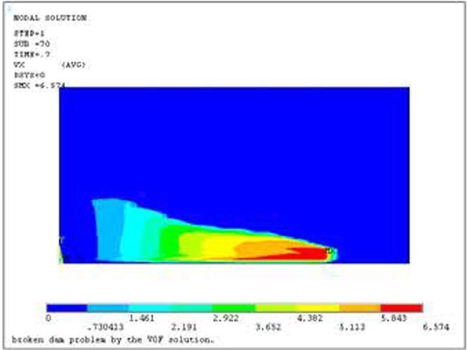
图7-72 流体横向速度场分布等值线图

重复第步操作。在“Item to be contoured”列表框中依次选择DOF Solution→Y-Component of fluidvelocity，单击“OK”按钮，ANSYS窗口将显示如图7-73所示的流体纵向速度场分布等值线图。

图7-73 流体纵向速度场分布等值线图

依次选择Main Menu→General PostProc→Plot Results→Vector Plot→Predefined，会弹出“Vector Plot of Predefined Vectors”对话框，如图7-74所示。在对话框中选择“DOF Solution→Velocity V”，单击“OK”按钮，会得到流场的速度分布图，如图7-75所示。

图7-74 “Vector Plot of Predefined Vectors”对话框

图7-75 流场的速度分布图